Written by Karan Beeshm
Sunday, July 26, 2026
Simulating Ice Thermal Storage Systems - Part 01: How Ice Thermal Storage Systems Actually Work
By
Karan Beeshm

Cooling Doesn’t Have to Happen When You Need It
Cooling a building doesn’t have to happen at the same moment a building needs it.That’s the entire premise behind ice thermal storage (ITS): instead of running a chiller flat-out every time occupants need cool air, you let the chiller do its work overnight — when electricity is cheap and outdoor conditions are mild — and bank that cooling as ice. During the day, you spend down the “cold” you already paid for.
It’s a simple idea with real operational upside: lower on-peak electricity draw, smaller peak chiller loads, and more flexibility in how a building’s cooling plant is sized and dispatched. But simple ideas can still be hard to model accurately. In this post, we walk through how advanced simulation platforms like BuildingsAI represent ice storage systems — from the physical components involved, to the actual equations EnergyPlus solves under the hood.
What’s Actually in an Ice Storage Plant
A typical ice storage system isn’t a single piece of equipment — it’s an integrated plant with a few key components working together:
- A water-cooled or air-cooled chiller
- An ice storage tank containing the latent storage media
- Primary and secondary chilled-water pumps
- Distribution piping and control valves
- Building cooling coils or terminal units
The storage tank is the heart of the system. Think of it as a thermal battery: during charging, the chiller pulls heat out of the tank until ice forms around the internal heat exchanger surfaces. During discharging, warm water returning from the building flows through the tank, melts the ice, and comes out the other side as chilled water ready to serve the building.
The reason ice storage is so space-efficient compared to, say, a giant chilled-water tank, comes down to one physical property: latent heat of fusion. Instead of storing cooling by changing a fluid’s temperature (sensible storage), ice storage exploits the energy required to change water’s phase — from liquid to solid. That phase-change energy is enormous relative to a simple temperature swing, which is why ice tanks can store a lot of cooling capacity in a comparatively small footprint.
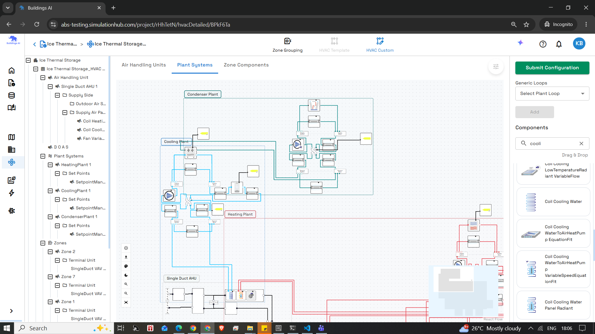
Chilled water loop branch showing the detailed ice storage tank plumbed in series with the electric chiller in BuildingsAI
Two Modes, One Tank
Ice storage systems operate in exactly two states.
Charging Mode
Charging happens when the refrigeration plant produces water or brine below the freezing point of the storage medium, gradually converting liquid water in the tank into ice. EnergyPlus tracks this using manufacturer-supplied performance curves that relate the charging rate to three things: how much ice is already stored, the log mean temperature difference (LMTD) across the tank, and the normalized mass flow rate. Charging continues until the tank is full or the scheduled charging window ends.
Discharging Mode
Discharging is the mirror image: warm return water enters the tank, absorbs latent heat as ice melts, and exits cooled. As the available ice shrinks, the tank’s cooling capacity gradually changes too — which is why EnergyPlus uses a separate set of discharging curves rather than just reversing the charging equations. The detailed model also includes an internal bypass: if the tank has more cooling capacity available than the load actually needs, part of the flow skips the tank entirely so the outlet temperature lands exactly at setpoint without wasting stored ice.
Why an Empirical Model, Not First-Principles Physics
Here’s a detail that surprises a lot of engineers the first time they dig into this: Energy Plus’s detailed ice storage object doesn’t simulate ice crystal growth, phase interfaces, or transient conduction inside the tank at all. Instead, it uses an empirical performance model — curves fitted directly to manufacturer test data.
This is a deliberate design choice, not a shortcut. Whole-building energy simulation needs to run a full year of hourly (or sub-hourly) timesteps in a reasonable amount of time, across potentially dozens of coupled systems. Solving detailed phase-change heat transfer equations for every ice tank, every timestep, isn’t computationally practical — and it isn’t necessary, because manufacturers already characterize their tanks’ real-world performance through lab testing. The empirical curves capture all of that nonlinear, real-hardware behavior without requiring the simulation to derive it from scratch.
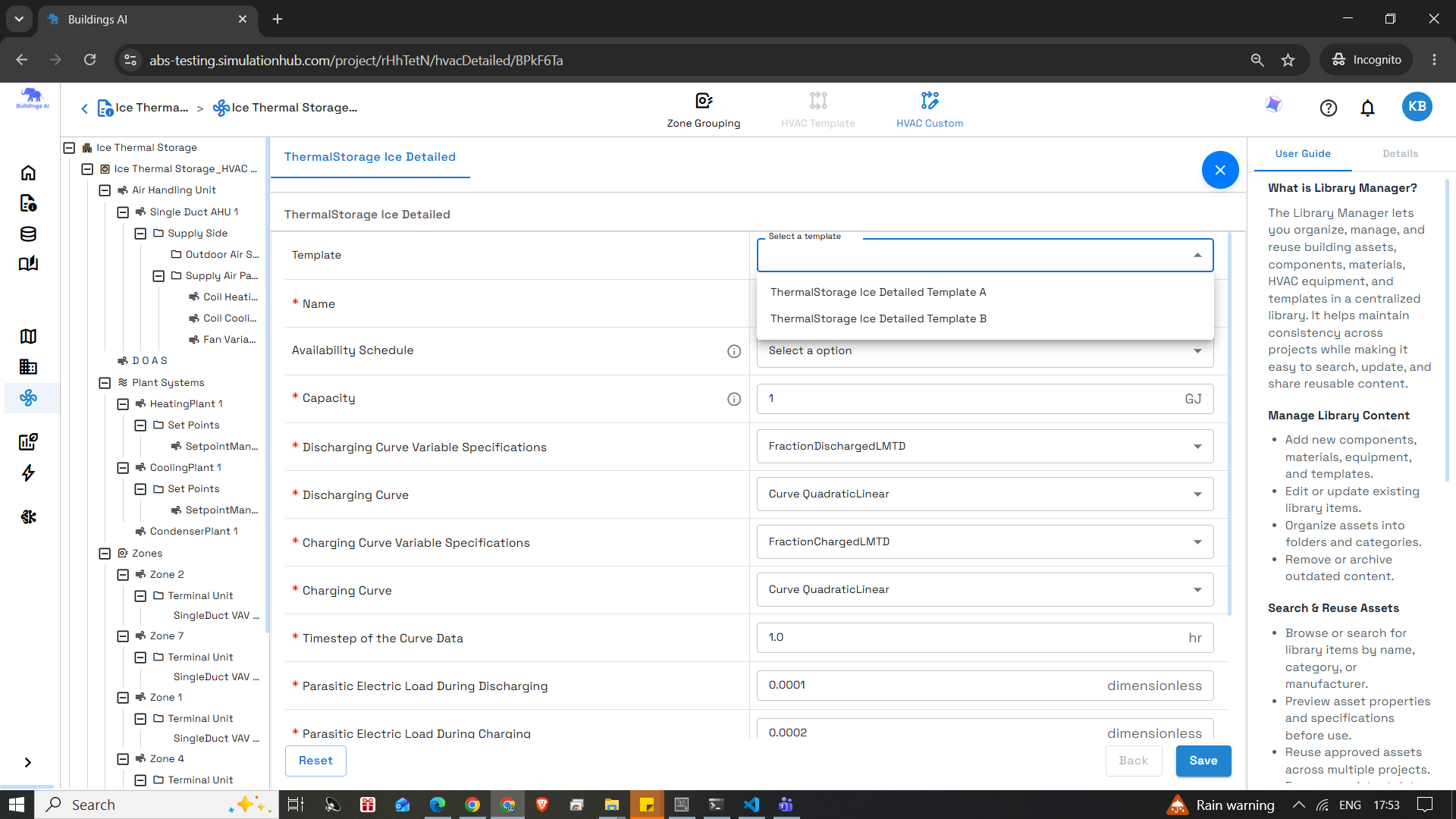
The detailed ice storage object configuration screen in BuildingsAI, showing charging/discharging curve selection, capacity, and parasitic load inputs
The Governing Equations
With that context, here is the actual math EnergyPlus solves.
Equation 1: Dimensionless Heat Transfer Rate

Where q is the instantaneous heat transfer rate (W), ∆t is the curve-fit timestep (typically 1 hour), and Qstor is the total latent storage capacity (J). Normalizing the heat rate this way means the same performance curves can describe tanks of different sizes — you just plug in a different storage capacity.
Equation 2: Log Mean Temperature Difference (LMTD)

LMTD represents the effective driving force for heat transfer between the circulating fluid and the ice. As inlet and outlet temperatures get closer to the freezing point, that driving force naturally shrinks. Because the performance curves are dimensionless, EnergyPlus normalizes this value too:

Equation 3: Charging Performance Curve

Here, Pc is the fraction of the tank already charged, and C1 through C6 are manufacturer curve coefficients. As ice builds up, the changing ice thickness alters heat transfer — but rather than modeling that geometry directly, those nonlinear effects are baked into the empirical coefficients.
Equation 4: Discharging Performance Curve

Structurally, this looks almost identical to the charging equation — but manufacturers typically supply different coefficients here, because melting ice and freezing water don’t behave the same way thermally
Closing the Loop: The Energy Balance
Once the dimensionless heat transfer rate is known, EnergyPlus still needs to translate that into an actual outlet temperature and heat transfer rate using the plant’s energy balance:

The tricky part is that the storage equation and the energy balance share two unknowns — outlet temperature and heat rate — so EnergyPlus solves them together, iteratively: it guesses the outlet temperature (starting from the scheduled setpoint), computes the LMTD, evaluates the performance curve for q, updates the outlet temperature via the energy balance, and repeats until the numbers converge. During discharging, the bypass logic layers on top of this same iterative process to make sure the tank isn’t over-discharged when it doesn’t need to be.
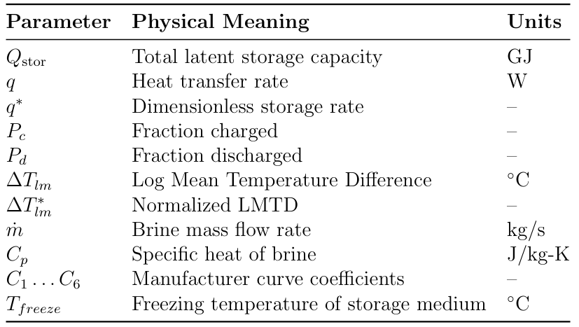
Model Parameters at a Glance
Why This Matters
Because the detailed model is built on manufacturer-specific curve coefficients rather than generic assumptions, it can represent real commercial ice storage tanks with meaningful accuracy — without sacrificing the computational speed needed for full annual building simulation. That combination is what makes it possible to actually trust the results when you use a system like this to evaluate a design decision.
Understanding the model is one thing. Seeing how it behaves inside a real building — with real climate data, real loads, and real utility rates — is another. That’s exactly what the companion case study covers next, using a mid-rise apartment building in Chicago.
What's Coming in Part 2
With the model and equations covered, Part 2 puts BuildingsAI to work on a real building:
- Building & Climate — a 7-zone Chicago apartment, sized against ASHRAE design days to stress-test charging and discharging.
- Plant Configuration — how the chiller, ice tank, boiler, and cooling tower are tied together in BuildingsAI, including the schedule that triggers charge vs. discharge.
- Comfort Results — full-year setpoint and comfort data across all zones.
- The Cost Payoff — on-peak vs. off-peak electricity savings, landing at a ~40% chiller cost reduction.
If you're evaluating ice storage for your next project, Part 2 is where the numbers get real.
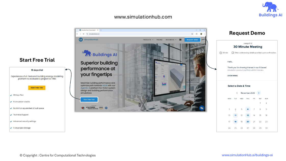
Take the Next Step: Start Your Free Trial or Book a Demo
Comments
Recent posts
Message
Dummy Name
Subscribe Newsletter
Register for Webinar
Sign up for AHC
App Dashboard
Buildings AI
Maximize building performance and path towards NZEB with our cloud-based, AI powered whole building performance modeling software.

Autonomous Valve CFD
Get CV, KV performance curves within minutes for your valve design. An automated CFD simulation based app for control valve designers.

Autonomous HVAC CFD
Leverage the power of autonomous HVAC CFD to design an efficient HVAC system for achieving indoor air quality and occupant thermal comfort.