Getting started with
Autonomous Valve CFD
Introduction to Autonomous Valve CFD app
What is control valve performance curve?
Every process plant consists of four main components, 1) Devices which generates the flow 2) Devices which carry the fluid from one location to other 3) Devices which control the quantity of fluid flow and 4) Devices which combines different fluids and generates the required product. The most common control element in the process control industries is the control valve. The control valve manipulates a flowing fluid to compensate for the load disturbance and keep the regulated process variable as close as possible to the desired set point. Control valves are playing a vital role in modern manufacturing process industries around the world to generate quality products.
The flow rate through a valve is controlled by manipulating the amount of open passage available for fluid flow. The amount of available fluid passage varies from 0% (fully closed) to 100% (fully open). The flow passage variations are achieved by a set of fixed and moving elements (also referred as valve trim) in the control valve.
The relationship between the valve stem (moving parts) position and the flow rate through a control valve is described by a curve called the valve's flow characteristic curve, or simply the valve characteristic. Typically, these characteristics are plotted on a curve where the horizontal axis is labeled in percent of maximum travel and the vertical axis is labeled as percent maximum flow.
Control valve trim design and performance curve
The synergy between what is demanded and what is supplied with the valve can be achieved by re-shaping the valve trim to get desired valve characteristics. The operating parts of a valve which are normally exposed to the process fluid are referred to as 'valve trim'. Usually parts like stem, plug, disc, seating surface, etc. are called as valve trim. Valve trim is the physical shape of the plug and seat arrangement. The shape of the valve plug determines the flow characteristics of the valve.
Different valve characterizations may be achieved by re-shaping the valve trim. For instance, the plug profiles of a stem-guided globe valve may be modified to achieve the common quick-opening, linear, and equal-percentage characteristics. The inherent characteristic curve is a plot of the percent of valve opening vs. the percent of the maximum flow coefficient (CV). This is determined by measuring the flow rate at various positions of valve travel with a fixed differential pressure across the valve. The CV value is calculated at each valve position using a form of the generalized Control Valve CV equation.
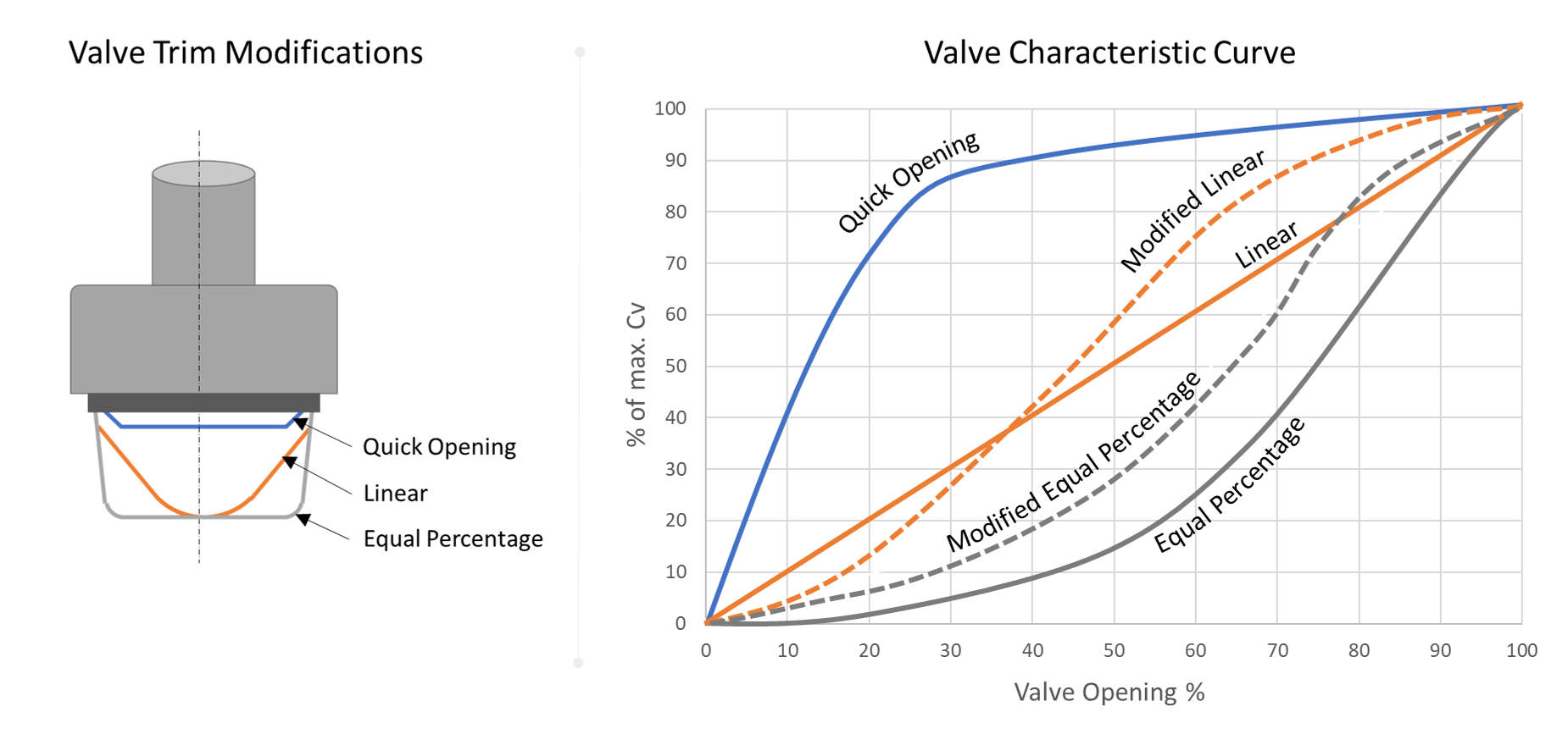
Quick Open : A quick opening valve plug produces a large increase in flow for a small initial change in stem travel. Near maximum flow is reached at a relatively low percentage of maximum stem lift. Quick open plugs are used for on-off applications designed to produce a maximum flow quickly.
Linear : An inherently linear characteristic produces equal changes in flow per unit of valve stroke regardless of plug position. Linear plugs are used on those systems where the valve pressure drop is a major portion of the total system pressure drop.
Equal Percentage : The equal percentage valve plug produces the same percentage change in flow per fixed increment of valve stroke at any location on its characteristic curve. The equal percentage is the characteristic most commonly used in process control.
Need for different trim design and characteristic curves
A control valve is a part of the complete fluid flow system. The fluid flow system may include other components like a pump, heat exchanger, reactor, piping, etc. Considering all other components in the system, it is necessary to achieve the desired flow characteristic curve. This is referred as installed valve characteristics.
Imagine that the process needs a linear increase in the flow rate. As pressure drop is the function of flow rate, the system pressure drop might be linear or non-linear depending on various components in the complete flow system. In case if the system pressure drop is also linear, a linear characteristic curve will satisfy the purpose. But in case if the system pressure drop is non-linear, we may need to go for quick opening or equal percentage control valve.
Hence, control valve trim is designed and manufactured in a variety of different characteristics to provide the desired installed behavior.
Computational Fluid Dynamics and Performance Curve
In order to select an appropriate control valve for process control, it is necessary to estimate the characteristic curve of each valve. The control valve design starts with a required maximum value of valve coefficient and its variation with the percentage of opening. Every valve design goes through design variation to satisfy required performance curve. Performance curve can be evaluated by measuring a flow rate vs. valve opening in a physical test setup. Doing such studies for each design variation is very time consuming and costly. Computational Fluid Dynamics is an effective alternative to evaluate performance curve during design stage for the control valve.

Computational Fluid Dynamics or simply CFD is an art / method / science / technique of solving mathematical equations governing different physics including a flow of fluid, a flow of heat, chemical reactions, phase change and many other phenomena. When applied to control valve performance curves estimation, it's about the solution of water flow equations in a control valve at various opening conditions. It helps valve designers to quickly calculate the valve coefficient, understand the flow behavior inside the valve and to optimize the design for required valve characteristics.
Traditionally, CFD is considered as a three step processes, viz. pre-processing, solving and post-processing the results. In case of control valve performance curve evaluation, pre-processing involves creating a 3D CAD model of a control valve, preparing CAD models for CFD meshing, creating a mesh inside a valve, creating solution setup and solution of flow equations. After the solution of flow equations, flow rate across the inlet and outlet of a valve is calculated to get valve coefficient. This process is then repeated for different opening position to get a performance curve.
Few of the major obstacles for using CFD in control valve performance calculation includes the complexity of valve geometry, compute power and time required for multiple opening conditions.
What is Autonomous Valve CFD app?
In a traditional way, calculating control valve performance curve using CFD involves the following process.
- For each opening position, creating 3D CAD model of control valve, extracting fluid domain and creating a CFD mesh.
- Doing required CFD setup and conducting analysis for number of opening conditions (typically between 5 to 10 depending on the accuracy of performance curve required).
- Combining a valve coefficient value and generating a performance curve.
The process needs CFD expertise, its compute-intensive and typically takes days to complete.
Autonomous Valve CFD (also referred as AVC) is a cloud-based Software-as-a Service (SaaS) from simulationHub, that uses CFD as a tool to simulate and plot the flow characteristic curve of a control valve. AVC is developed specially for design engineers and manufacturers to help them simulate the performance of their design,without having any knowledge of CFD. The app only needs a control valve geometry,number of opening conditions and flow direction. All CFD setup, calculation, and the result extracted is automated using specifically written algorithms for control valve performance evaluation.
All CFD computations are done using cloud computing. The app does not need any high-end local machine and even can be used for mobile / tablet devices. Once the setup is submitted from computation, ready-to-use valve performance PDF report is generated within few hours. The report includes all setup information, a valve characteristic curve, and more detailed CFD results. AVC application supports performance evaluation of rotary, lift and on/off type valves.
User interface

Following are the major components of Autonomous Valve CFD app interface:
1
Simulation details and help toggle button
:
Access the simulation details, help and support menu. This allows opening the simulation details page. A quick link to help items like getting started guide, video library and forum is given. You can also raise the support ticket for opening simulation.
2
Simulation stage navigation toggle button
:
This button toggles the stage navigation menu of left.
3
Navigation menu for an individual stage
:
A typical simulation includes a number of the main stages. Each main stage includes a number of sub-stages. For example, the location and wind condition stage have two sub-stages, location & wind rose and wind conditions for simulation. Navigation menu for an individual stage is available in the left navigation panel. Individual stage menus will change depending on the stage you have opened. For example, in result stage, you can view comfort plot, flow lines, surface pressure, contour plots, etc. Clicking on each sub-stage will open the respective sub stage options. This menu follows stage dependency and color coding.
4
Previous & next stage access
:
A quick access link is given to go to previous or next simulation stage. The access to the next stage is deactivated until the current stage is completed. This menu follows stage dependency.
5
Stage quick access
:
Stage quick access is available at bottom of stage navigation panel. This quick access helps to navigate between main simulation stages. This menu follows stage dependency and color coding.
6
View cube
:
Use the View cube to orbit your design or view the design from standard view positions. If you hover on the view cube, you can see a drop-down icon in a bottom right corner with more view options.
7
Model view controls and settings
:
The model view controls contain commands used to zoom, pan, and orbit your design. The display settings control the appearance of the interface and how a model is displayed in the graphics window. You can also take the snapshot of what is displayed in the graphics window.
8
Model click menu
:
Left-click to select the object in the graphics window. Right-click to access the model menu. The model menu contains commands like to isolate, hide selected, show all objects. Left click anywhere in the graphics window to hide the model menu.
9
Results quick access menu
:
Results quick access menu is available when you open the result state of the simulation. This quick access menu helps to navigate to different results without using the left navigation panel. A quick access menu contains commands to go to results like comfort plot, flow lines, contour plots etc.
10
Profile and help
:
In profile, you can control your profile and account settings, or use the help menu to continue your learning or get help in troubleshooting. This menu also contains a quick link to the dashboard. Use the full - screen icon if you wish to use the app in full-screen mode.

Mobile device modifications

View cube 6 and result quick access 9 menus are not available on mobile and tablet. A profile and help menu 10 is modified for mobile and tablet devices. You will see raise ticket and sign out buttons in the profile and help menu. Model view control and settings 7 menus are also modified and available with fewer options.
Stage dependency and color coding

All the simulation stages are arranged in the sequential way they are executed. Every stage is dependent on the status of its previous stage. If the previous stage is not completed/failed, the stage will not be activated. This helps to complete the simulation stages in a sequential manner and avoid input errors.
The status of every stage/sub-stage is represented by unique colors. Green color indicates running stage, blue color indicates completed stage, black color indicated active stage, light grey color indicated deactivated stage and red color indicated the failed stage.
Create simulation
Create a new valve performance study by following below steps:
1
Create New Simulation
:
Click the "Create New Simulation" button on the dashboard. This will open up "Create New Simulation" popup window. (NOTE: The button will be deactivated in case if you do not have a valid app subscription.)

2
Simulation Details
:
Provide simulation name and description in giving fields. If you have only one app subscription, the app will automatically be selected in the template drop-down. In case of multiple app subscriptions, select the app template.
3
Create Simulation
:
Click 'Create Simulation' button. This will create a new simulation with provided details and open the 3D viewer for further setup.
Valve geometry
Once a new simulation is created, you will be directed to the geometry stage. This is the first step towards running a CFD simulation in Autonomous Valve CFD app.

Follow the steps below to upload valve geometry in the simulation project:
1
Input CAD Model
:
Click "Input CAD Model" in valve geometry and settings stage. This will direct you to sub-stage menu for the input CAD model.
2
Browse
:
If you have the geometry available on your local computer, click the 'Browse' button. This will open an 'Upload Local Geometry' dialog box. (NOTE: If you have geometry available on cloud storage, provide the link to geometry file and click 'Upload' under 'Upload Cloud Geometry' section. Currently, only Amazon S3 cloud storage links are supported).
As a directive to preparing the correct CAD model for the simulation, a special info titled Click here for the guidelines on "Preparing the CAD model" has been added.
3
Choose a File
:
Click on 'Choose a file to upload' button to open a file browser. The app currently supports ipt, IGES, STEP, SAT file formats. Select the file and click 'Open' in the file browser. The selected file name will appear below the button.
The uploaded geometry should have an appropriate position of a moving component (trim). If you wish to evaluate flow performance at various opening angles (flow regulation or control valve), you need to update the geometry in fully closed condition. If you wish to evaluate flow performance only at one opening condition (isolation or ON-OFF valve), you need to update the geometry in fully open condition.
4
Upload
:
Click "Upload" button to upload the file to your simulation. The time required to upload the file will depend on the size of a file. Once the file is uploaded, the 3D viewer will show the geometry and will direct you to the next stage. You can notice that the geometry stage is marked completed (blue color) in stage quick access menu available at bottom of stage navigation panel.
Once the valve geometry is uploaded, few details of valve need to be specified.These valve details help to characterize the uploaded valve geometry and do the appropriate setup during valve performance study.
5
Specify Valve Details
:
Click on 'Specify' button under the Provide Valve Specification menu. This will open a Valve details dialog box wherein you can specify your valve details. In the Valve Details dialog box, you will have to specify the Valve function, plug motion type, valve type, valve size, pipe schedule, pressure class,design Cv (optional), body material and trim material. You can also add an image of the valve (optional). After entering the valve details, click on the 'Apply' 6 button.

Moving parts settings
To get the performance curve for rotating or lift control valve, the user needs to define valve opening conditions. Opening settings define moving parts of valve trim, an axis along which parts will move and the number of opening conditions.
1
Moving part settings
:
Click "Moving Part Settings" in main Valve Geometry and Settings stage. This will direct you to sub-stage menu for selecting moving parts of a control valve.
2
Start selection
:
In this stage, the user will have to select the moving parts of the valve for the valve geometry by clicking on 'Start Selection' button under the Rotating/Lifting Parts section.

3
Add body to moving bodies
:
Left click and select the moving parts of the valve (disc/ball/plug/shaft/etc...) from geometry loaded in the viewer, then right click and select 'Add body to moving bodies' from the options. Repeat the same for all the moving bodies in your geometry. You can also add multiple bodies simultaneously by pressing the 'CTRL' button on the keyboard while selecting the bodies.
4
List of Selected bodies
:
This box will show a list of selected objects and user can hide or remove selected objects from options given.
5
End Selection
:
Once all the moving bodies are selected, click on 'End Selection' button for confirmation that all moving parts have been added.
Axis of motion
1
Select Axis
:
An axis is required to provide motion of valve moving parts.The options are available under the 'Axis of Rotation/Lift' section on the left navigation panel. This method is the same for rotational and lift valve.


2
Select a method
:
There are two methods available for selecting an axis for the control valve. Choose one from the drop-down menu.
1
Axis using cylinder
:
This method involves selecting an axis of rotation/lift for the moving bodies by selecting a cylindrical surface through which the axis will pass.
Choose 'Axis using cylinder' from the drop-down menu.
Click on 'Select cylindrical surface'. Select the cylindrical surface on the geometry through which the axis will pass. Shaft surface would be
appropriate for all the cases. Refer 3 A dotted axis will appear passing through the center of the cylinder you selected.
2
Axis using two points
:
This method will be used if the user could not find any concentric cylindrical surface through which the axis passes. Here you can select two surfaces such that the axis will pass through their centers.
Choose 'Axis using two points' from the drop-down menu.
Click on 'Select start point surface(s)', select the first surface on the geometry through which the axis will pass. Click on 'Accept'. The point will be created at the center of the selected surface.
Click on 'Select endpoint surface(s)', select the second surface on the geometry through which the axis will pass. Click on 'Accept'.
A dotted axis will appear between the two centers of the surfaces selected.
Valve opening conditions
A complete performance curve for a valve contains valve coefficients from fully closed to a fully open condition. The accuracy of the performance curve depends on the number of opening conditions considered for performance evaluation. Typically, 5 to 10 number of opening conditions are considered good for an accurate representation of valve performance curve. Autonomous Valve CFD app provides user to run the simulations the number of conditions anywhere between 1 to 18.

To avoid simulation failure, it is recommended to provide opening conditions anywhere between 20 % to 100% opening of a valve in.
In case of rotation motion type, provide minimum and maximum opening angle. The Minimum angle should be more than or equal to 20° and the maximum angle should be less than or equal to 90°.
The methodology of specifying openings is the same for rotation motion type and linear motion type valves. Firstly, provide the maximum rated opening of the valve. For linear type provide the maximum opening in cm while for rotary type provide the maximum opening in degree of angle. For rotary type the maximum rated opening is 90 degree while for linear type the maximum rated opening is 3 times of the valve diameter specified in valve details.
Once you specify the maximum rated opening, choose if you want to run for multiple openings or single opening.
Once minimum and maximum rotation/lift conditions are provided, enter the total number of opening conditions. The opening conditions will be equally divided between the minimum and maximum opening value. For example, if the minimum opening is 20%, maximum opening is 100% and the number of conditions is 9, the opening angle for simulation will be 18°, 27°, 36°, 45°, 54°, 63°, 72°, 81° and 90°. Selection procedure for valve opening condition is given below.
1
Specify rated opening
:
Enter the maximum valve opening condition (for Rotating valve it should be in degrees of angular rotation and for linear valve should be in a centimeter of displacement.)
2
Creating opening conditions
:
Click to create the opening conditions to be simulated. A pop up appears in which you need to specify whether you want to run multiple openings or single opening. Multiple opening is selected by default. Edit the minimum and maximum opening conditions, the number of steps desired.
3
Add conditions
:
Click apply and the number of openings is added to be simulated.
4
and
5
Preview and Apply settings
:
You can preview the valve opening conditions to confirm the opening settings. Make sure that the valve rotates or translates in the correct direction. If the rotation or translation is in the opposite direction, tick on the reverse direction checkbox and check for preview.
6
Save opening settings
:
Click 'Apply' button to save opening conditions. These conditions will then be saved with valve performance study.
Click on the next stage to proceed further.
Valve connections
To do CFD simulation at each opening position, flow direction needs to be specified. Valve connection settings allow you to specify the inlet and outlet side of the connecting pipe which determines the direction of flow.

Following is procedure define inlet and outlet connections:
1
Connection Settings
:
Click on 'Define Valve Connections' from stage 'Valve Connections', this will open the sub-stage menu in Valve connections. Here the user needs to select inlet/outlet connection by choosing appropriate pipe connections from uploaded the geometry.
2
Select Inlet Pipe
:
Click on 'Select Inlet Pipe' button. Then select inlet pipe connection by clicking 3 on to the inlet pipe geometry.
4
Select Outlet Pipe
:
Click on 'Select Outlet pipe' button. Then select outlet pipe connection by clicking 5 on the outlet pipe geometry.
Color codes are given to identify connections.
Indicates probable inlet/outlet faces
Indicates selected Inlet Connection
Indicates selected Outlet Connection
6
Save Connection settings
:
Click "Apply Connections" button to save the applied valve connection settings.
The flow will now be simulated in the direction defined based on the inlet and the outlet connections.
CFD simulation
Autonomous Valve CFD app uses cloud computing for all calculations. The process will include meshing, solving the numerical equations and finally post-processing of the results.

To submit the simulation run and check status, do the following:
1
Simulation Run
:
Click on "Simulation Run and status". This opens a sub-stage for submitting the simulation and checking the status of the simulation.
2
Submit Simulation
:
By clicking 'Submit Simulation' to open the 'Run Simulation' dialog box.
3
Run Simulation
:
The 'Run Simulation' dialog box informs you about the number of simulation credits that are to be consumed for your current simulation. It also provides the total credits available in your account. Click on the 'Run Simulation' button to begin the simulation.
The Autonomous Valve CFD app will now begin with the process to generate the fluid volume, mesh, run the simulation and perform post-processing on the results.
3
Check Status
:
In the left Navigation Panel, the status of the simulation will be shown under the 'Simulation Status' section. The time required for simulation depends on the size of geometry and number of opening conditions submitted. Simulation of each opening conditions has different stages. Live feed of each stage statues will be shown for all opening conditions. Once the simulation is completed, progress bar for each opening condition will be marked with blue color and overall status will be marked "Completed". The user will be notified about the completion of the simulation on his registered email id.
5
Terminate
:
In case you wish to stop your simulation in between, you can click on the "Terminate" button. The simulation will stop immediately. You can make the necessary changes once the simulation is terminated.
Note: If in case you make changes in the Valve Connections stage on an already completed simulation, the 3Run Simulation dialog box will reappear and inform you about the simulations credits to be consumed.
Flow lines
Flow lines depict the path followed by fluid particles from an inlet to the outlet of a valve. The animated arrows on the flowlines indicates direction of velocity vectors at that point and speed is based on the magnitude of velocity. This is similar to the flow visualization technique where some colored particles are injected from an inlet and its trace in the flow domain is marked. Along with that path, the flow lines also display the magnitude of velocity and pressure of each particle along its path. This is useful information to identify flow separation and recirculation zones in a valve.
Click on the 'Results' stage from the stage quick access menu to open the results page, where options to access different results are listed in the left navigation panel.You can access the flow lines by clicking Flow Lines in 'Results' main stage or by using 'Results quick access menu' provided at the top center of the 3D viewer.(NOTE: If you have not gone through the 3D results user interface, it is strongly advised to refer to 'User interface' section and get familiar with the interface of 3D results).

Flow lines are loaded with the default configuration of an opening condition, variable, colors, and opacity. Use following settings to modify the display of flow lines:
1
Variable
:
Select the variable to be used to color flow lines. You can select either velocity or pressure as a variable. You can also change the number of color bands to be used to create the color variation. By default, variable variation is shown using 16 colors. Anywhere between 2 to 100 colors can be used as a color variation. Change the variable, change the number of colors and click "Apply" button. This will apply selected change on the colors of flow lines.
2
Model opacity
:
To get a better view of flow lines, the model is made translucent while loading flow lines. You can change the opacity settings using the slider provided in 'Model Opacity' section with 0 indicating fully transparent and 1 indicating fully visible. In case if you have a multi-part model, you can change the opacity of one / more parts. Check the 'Selected Only' option, select single / multiple parts and drag the opacity slider. Drag and release the slider at desired opacity to change the opacity of model. Click 'Reset' button make model fully visible.
3
Color legend
:
CFD analysis generates a numerical data as a result. The understanding large quantity of numbers is very difficult. To give a better understanding of results and to create a visual representation of numbers, a color coding method is used. The range of minimum to the maximum value is first divided into the number of groups (In simulationHub, we divide them 2 to 100 groups). Each group is then assigned a unique color. Any number then gets a color based on which group it belongs to. In simulationHub, we use a color variation between blue to red where blue indicates a minimum value and red indicates a maximum value. The color legend shows the minimum and maximum value, variable displayed and color for each group.
4
Take a snap
:
Click 'Set simulation image' button located in a menu at mid-bottom of the viewer. This will open a 'Take a Snap' dialog with image preview. 'Set as simulation feature image' option will make the snap as simulation feature image display on the dashboard and the simulation details page. 'Add in simulation repository' option is used to keep the snap in simulation data for future reference. 'Download Image' option should be selected to save the image in your local device storage.
5
Change valve opening
:
For a lift and rotating type control valve, the number of opening conditions is used to get the complete performance curve. The number of opening conditions depends on the performance curve accuracy required and can be selected anywhere between 2 to 8 while doing opening settings.
A performance curve is a single curve generated considering all opening conditions. Other CFD results like flow lines, flow lines with vectors and contour plots are available for each opening condition. You can view and analyze these results to see flow features for each opening angle and take a decision on design modifications to get the desired performance curve.
By default, flow line results are displayed for the minimum opening condition. To see flow lines for other valve openings, click on "Select condition" drop-down, select a desired opening condition from the list and click "Apply" 6 button. his will display the flow lines for the selected opening condition.
6
Settings
:
Flow lines with animated velocity vectors are loaded as default. User can ON/OFF visualization using checkbox and animation speed can be adjusted/scaled anywhere between 1 to 100 using speed slider.
Surface pressure
Surface pressure is pressure contours plotted on the surfaces in contact with the fluid. This information is useful to identify the regions of low-pressure zones and the possible locations of flow recirculation.
To access the surface pressure, click Surface Pressure in result main stage. You can also access this using "Results quick access menu" provided at the top center of the 3D viewer.

Surface pressure is loaded with the default configuration of an opening condition, variable, model opacity, and surface visibility. Use following settings to modify the display.
1
Variable
:
"Color By" drop-down is deactivated as surface pressure plots are generated only with pressure values. By default, the 16 number of colors are used to display the surface pressure plot. To change the number of colors, drag and release the color slider at a desired value and click "Apply" button.
2
Model opacity
:
To get a better view of surface pressure plots, all the model parts are made hidden. To view the geometry along with surface pressure, right-click anywhere in the graphics window and select "Show all objects". You will see now see the geometry along with surface pressure. You can then adjust the opacity of geometry using the Opacity slider in "Model Opacity" section.
6
Surface visibility
:
To get a view of pressure on internal surfaces, sometimes it is needed to hide pressure plot of few surfaces. You can use the options in "Surface Visibility" section to hide surface. Click on "Select Surface" button, select the surfaces you want to hide, click on "End Selection" button to end the surface selection process. All the selected surfaces are shown in "Selected Surface" table. Use / icon to hide/show the individual surface. Click icon to remove surface from the selection list. You can use / icons in the table header to hide/show all surfaces and icon to remove all the surfaces from the selection list.
Usage of 3 Color legend, 4 Take a snap, and 5 Selection condition are same as that of flow lines results.
Contour plots
The contour plot is a pictorial representation of flow property variation in the fluid domain. The location of flow separation, high velocity, and low-pressure regions are few examples of insights that can be gained through CFD results visualization. Contour plots display the velocity or pressure variation about any 2D cut section of the geometry.
To access the contour plot, click Contour Plots in 'Results main' stage. You can also access this using "Results quick access menu" provided at the top center of the 3D viewer. Contour plots loads with default settings for an opening condition, cut plane location, variable and model opacity. Use following settings to modify the contour plot.

Usage of 1Variable, 2Model opacity, 3Color legend, 4Take a snap, and 5Opening condition is same as that of flow lines results.
6
Cut plane
:
Contour plots can be shown in X, Y, or Z direction. To change the cut section direction and location, sliders are provided in "Cut Plane" section. You can change the plane location from 1 to 100 where 50 represents the middle cut section.By default, Z = 50 cut section is displayed. The displayed cut section value and direction is shown at the bottom. To change the cut section, drag and release the slider at the desired location.
7
Settings
:
When the cut section is selected for contour plot, the geometry is also sectioned at the selected location. This shows only one side of the geometry to make contour plot visible. If you want to get the full display of geometry, you can deactivate "Section Geometry" option in the settings section.
Performance data
Autonomous Valve CFD app generates various valve performance data including valve coefficients like Cv, Kv, K and Cdt at various opening conditions. Flow performance coefficients (Cv, KV) are determined based on the procedures prescribed by the IEC & ANSI standards. The Cv value is calculated as a function of both the line flow rate and the pressure drop across the valve. The app provides valve flow performance coefficients in both Gross as well as Net values.
The Gross Cv incorporates the complete pressure drop of the pipe connections as well as the valve whereas, the Net Cv incorporates the pressure drop across the valve excluding the pressure drop due to valve.
To access the performance data, click Performance Data in ‘Results’ main stage. You can also access the performance data using ‘Results quick access menu’ provided at the top center of the 3D viewer. All the performance data is shown in the left panel.

1
and
2
Result summary
:
Result summary contains tables and charts of the valve performance coefficients. Using the checkboxes given user can select between the value to be shown in “Gross” or “Net” format. This summary includes CV, KV coefficient values and pressure drop at various valve opening conditions, K head loss coefficient and coefficient of hydrodynamic torque (Cdt) for the rotating motion valves.
3
Detailed Results
:
To visualize the gross and net values simultaneously click on detailed results. A table will pop which will show both the performance coefficients for gross as well as net values.
4
Export Result
:
The detailed results can be exported results in CSV (comma-separated values) format, by clicking on the ‘Export Result Summary’ button. You can export these results in CSV (comma-separated values) format, by clicking on the ‘Export Result Summary’ button. You can open this .csv file in many software like Microsoft Excel, OpenOffice or Google Docs to create your custom graph.
5
Valve Cv curve
:
Based on your selection in step 1 as gross or net data, this section shows the valve flow coefficient - CV curve which is a plot of opening configuration on X-axis and CV values on Y-axis. By default, the gross CV values are displayed. You can choose to display net CV values as well.
6
View & export plot
:
To see the enlarged view of the plot, click on the ‘View & Export button’. This will open a CV Curve dialog box. Mouse over on any data point will show exact value of opening condition and valve coefficient. To export the curve, click on ‘Export’ button 7 in the ‘CV Curve’ dialog. This will open an ‘Export’ dialog box. The coefficient curve can be exported in a CSV file format or as a PNG image. You can export images in different resolutions – regular/HD-ready/Full-HD/4K/5K resolution. Select a desired export option and click on ‘Export’ button. This will download the result in selected file format.
Kv coefficient 8, K 9 and Cdt 10 curves are presented in the left panel. Use the same procedure as above to view and export these results.
Valve performance report
Autonomous Valve CFD app comes with a unique report generation feature. We have extracted required and critical information about analysis to compile a ready-to-use PDF report. The report begins with an executive summary including a quick view of performance curves. The following section contains details like simulation name, objective and view of a CAD model of a valve. The CFD section gives you information overall methodology used, fluid properties and assumptions made during CFD analysis. The result section starts with quantitative results including Cv, Kv coefficients at all opening conditions. It also includes performance plots. The qualitative results include velocity and pressure contour plots at mid-section for all opening conditions.
To access the CFD analysis report, click Report in 'Results' main stage. This will open a PDF report window. You can download the report using download button provided in the top right menu.
To provide a detailed explanation on calculation of gross and net values, an annexure has been added to the report.

NOTE : Once the simulation is completed, a PDF document of the report is also sent as an attached to simulation completion email.
Dashboard

Once you log into the simulationHub account, the user would be directed to the dashboard. In general, one can click on the dashboard icon or use the link in the top navigation bar to open dashboard.The dashboard provides an at-a-glance view of all your simulations.The dashboard contains main components like a top navbar, sidenavigation, simulation quick-view tile and other important information about your account and subscription.
Simulation quick-view tile on the dashboard has following components:
1
Simulation image
:
The simulation image on dashboard tile gives a quick visual view of simulation. This image is automatically updated based on the recently opened / completed simulation stage. You can also set this image using "Set simulation image" button available in the 3D viewer. Click on the simulation image will open simulation in the 3D viewer.
2
Simulation details
:
Simulation details section on quick-view tile contains information like simulation name, simulation app, and last opened / edit information. By default, all the simulations are arranged in descending order of its last access time.
3
Simulation status
:
Simulation status is the dynamic content of quick-view tile. The progress percentage, status and progress bar will change based on the status of the simulation. Appropriate color coding is used to give the visual representation of simulation status.
Quick links are provided to open
4
details page or 5
3D viewer of the simulation.
Simulation details
Simulation details page contains all the information either entered by you or generated during the simulation process. We have written app specific algorithms to extract all the simulation information and presented in a report ready format.
1
Name and details
:
Simulation name and details are provided at the top.
2
Simulation image
:
The image slider contains all the simulation images. These images are automatically updated based on the recently opened / completed simulation stage. You can also set this image using "Set simulation image" button available in the 3D viewer.
3
Simulation details
:
The simulation details section contains all input information including name, description, valve type, opening conditions, etc. The simulation results information is arranged in different sections. It first includes the valve performance summary, CV, KV and pressure drop performance plots. The CFD results are presented in the different section and include image sliders for specific output like flow lines, flow lines with vectors, contour plots etc. You can collapse the view of each section using the arrow provided at the top right corner of each section.

4
Simulation actions
:
Simulation action section provides buttons to perform different actions on the simulation. You can open 3D simulation, copy, edit or delete the simulation using these buttons.
5
Quick glance
:
The quick glance section contains some important information about simulation. It includes simulation details, overall simulation status, simulation images and important notifications about the app.
6
Left navigation toggle button
:
This button toggles the left navigation menu. The left navigation menu contains simulation filter (recently opened / filter by app / simulation gallery), help and support section and account section. You can access app specific help or raise a support ticket for your simulation.
6
Profile and help
:
In profile, you can control your profile and account settings, or use the help menu to continue your learning or get help in troubleshooting. This menu also contains a quick link to the dashboard. Use the full-screen icon if you wish to use the app in full-screen mode.
Mobile device modifications

A profile and help menu 7 is modified for mobile and tablet devices. You will see raise ticket and sign out buttons in the profile and help menu.
Geometrical preparation guidelines
simulationHub Valve CFD app has been developed such that, it makes the process of
running a CFD simulation using the input valve CAD model very user-friendly.
simulationHub supports a variety of different file formats, including standard formats
like STEP and IPT. This makes the app compatible with most of the available CAD
software. The app also takes care of the CAD repair required for running a successful
and failure-free CFD simulation.
Here are some guidelines to ensure that the uploaded geometry is ready for the simulation in the simulationHub Valve CFD app.
1
CAD Assembly and File Format
:
Upload the input CAD model as an assembly file or a multi-body part file. The current version of
simulationHub support following CAD file formats: IPT, STP, STEP, SAT, X_T.
Each component in the CAD file should be a separate individual body/part i.e., disk/ball/plug,
stem, body, flanges, upstream pipe, downstream pipe, the seat should be maintained as a
separate body.

2
Pipe Connections
:
The image slider contains all the simulation images. These images are automatically updated based on the recently opened / completed simulation stage. You can also set this image using "Set simulation image" button available in the 3D viewer.
Attach pipe geometries :
Uploading only the valve geometry is incorrect. The CAD model should have pipes attached upstream and downstream of the valve.

Length of the pipe connections :
A pipe length of 2.5D is required at the upstream and
10D is required at the downstream side of the valve body.'D' is the valve size (to be
specified in the 'Valve Specifications' section).
Please note that the pressure measurements would be taken at 2D-6D locations as per the ANSI/ISA-75.02.01 standards

Pipe Diameter :
Both upstream and downstream pipes should have an internal diameter (ID), based on the valve size and the pipe schedule used in the flow loop test facility.
For example, pipe ID for a DN 300 valve size and schedule 40 can be determined from the table as:
Pipe ID = Pipe OD - (2 x Wall thickness)
Pipe ID = 323.85 - (2 x 9.525) = 304.8 mm
Note: It is suggested to do the calculations in 'mm' to avoid round off errors

For complete-dimension details of different valve sizes and pipe schedules, please refer https://en.wikipedia.org/wiki/Nominal_Pipe_Size
Water-tight Geometry :
CFD simulation needs a water-tight geometry. As this is taken care of by the app algorithm internally, it is suggested that the pipe ends in the input CAD model be kept open.
3
Valve Opening Position

Flow regulation or Control valve :
Upload valve in the fully closed position. Refer fig (a)
Isolation or On/Off valve: :
Valve should be uploaded in an open position, at which Cv is required. Refer fig (b)
Mobile device modifications
A profile and help menu 7 is modified for mobile and tablet devices. You will see raise ticket and sign out buttons in the profile and help menu.
Subscription plans
The Autonomous Valve CFD app has variety of subscription options suitable for different design and analysis needs. Explore the options and choose the one best suitable for you.
Free trial
We say it all. It's easy. It's efficient. It's built for designers. But you be the judge. Take a full version app trial for FREE. Try it on your own design problems and experience the power and benefits of the app.
Start Trial
Yearly subscription
Are you a busy designer? Do you work in an organization with frequent design load? Take our yearly subscription plan and enjoy uninterrupted app access and more simulation credits per cost.
Subscribe
Want to know more?
Want to know more about Autonomous Valve CFD app? Visit blogs and simulation gallery to get details of real life applications or simply schedule a demo with our expert.
Blogs
Read about an application of Autonomous Valve CFD for valve design. Learn about latest app features, tips, tutorials. Find out the views and opinions on design trends in control valve industry.
View blogs
Case studies
Autonomous Valve CFD app is used to design, develop and optimize control valve performance. Read the real-life industrial case studies about how the app is used to improve control valve performance.
Simulation gallery
Request demo
It's easy. It's powerful. It's built for designers. Learn how simulationHub apps can help you optimize your own product design. Schedule a one-on-one demo with a simulationHub expert.
Request demo